Introduction to Quantum Mechanics
Chapter 1 | The wave function
Schrodinger equation
- The wave function of a particle is got by solving Schrodinger equation: \[ i\hbar \frac{\partial \Psi}{\partial t}=-\frac{\hbar^2}{2m}\frac{\partial^2\Psi}{\partial x^2}+V\Psi \] where \(\hbar =\frac h{2\pi}=1.054\times 10^{-34}J\cdot s\).
Statistical interpretation
- Born's statistical interpretation:
 - Copenhagen (orthodox) interpretation: it's the act of measurement that forces a particle to "take a stand". The measurement radically alters the wave function of a particle and makes it sharply peaked around \(C\)(which is the result position of measurement).
Normalization
- We need the normalization to be consistent with the statistical interpretation
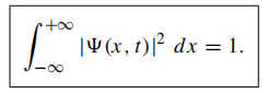 - The Schrodinger equation has the property that it automatically preserves the normalization of the wave function: \(\frac{d}{dt}\int_{-\infty}^{+\infty}|\Psi(x,t)|^2dx=0\) since \[
\frac{d}{dt}\int_{-\infty}^{+\infty}|\Psi(x,t)|^2dx=\int_{-\infty}^{+\infty}\frac \partial{\partial t}|\Psi(x,t)|^2dx,\\
\frac{\partial}{\partial t}|\Psi|^2=\Psi^*\frac{\partial \Psi}{\partial t}+\frac{\partial \Psi^*}{\partial t}\Psi.
\] Plug in the Schrodinger equation, we'll get \[
\frac{\partial}{\partial t}|\Psi|^2=\frac \partial{\partial x}[\frac{i\hbar}{2m}(\Psi^*\frac{\partial \Psi}{\partial t}-\frac{\partial \Psi^*}{\partial t}\Psi)],
\] and the integral will be \(\frac{i\hbar}{2m}(\Psi^*\frac{\partial \Psi}{\partial t}-\frac{\partial \Psi^*}{\partial t}\Psi)|_{-\infty}^{+\infty}\), which is 0 by the normalizable condition.
- The Schrodinger equation has the property that it automatically preserves the normalization of the wave function: \(\frac{d}{dt}\int_{-\infty}^{+\infty}|\Psi(x,t)|^2dx=0\) since \[
\frac{d}{dt}\int_{-\infty}^{+\infty}|\Psi(x,t)|^2dx=\int_{-\infty}^{+\infty}\frac \partial{\partial t}|\Psi(x,t)|^2dx,\\
\frac{\partial}{\partial t}|\Psi|^2=\Psi^*\frac{\partial \Psi}{\partial t}+\frac{\partial \Psi^*}{\partial t}\Psi.
\] Plug in the Schrodinger equation, we'll get \[
\frac{\partial}{\partial t}|\Psi|^2=\frac \partial{\partial x}[\frac{i\hbar}{2m}(\Psi^*\frac{\partial \Psi}{\partial t}-\frac{\partial \Psi^*}{\partial t}\Psi)],
\] and the integral will be \(\frac{i\hbar}{2m}(\Psi^*\frac{\partial \Psi}{\partial t}-\frac{\partial \Psi^*}{\partial t}\Psi)|_{-\infty}^{+\infty}\), which is 0 by the normalizable condition.
Momentum
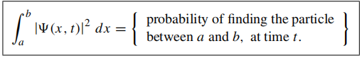
- For a particle in state \(\Psi\), the expectation value of \(x\) is \[ \langle x\rangle =\int_{-\infty}^{+\infty}x|\Psi(x,t)|^2dx, \] which is the average of measurements on an ensemble of identically-prepared systems.
Plug in the equation of \(\frac{\partial |\Psi|^2}{\partial t}\) we get previously and utilize integration-by-parts, we can get \[ \frac{d\langle x\rangle}{dt}=-\frac{i\hbar}{m}\int\Psi^*\frac{\partial \Psi}{\partial x}dx. \]
Let \(\langle v\rangle=\frac{d\langle x\rangle}{dt}\), we have \(\langle p\rangle=m\langle v\rangle=-i\hbar\int\Psi^*\frac{\partial \Psi}{\partial x}dx\).
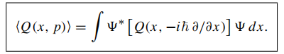
Defining the position operator as \(x\), the momentum operator as \(-i\hbar (\partial/\partial x)\), we can calculate the expectation of values by "sandwich" the appropriate operator between \(\Psi^*,\Psi\) and integrate.
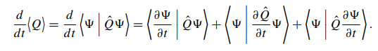
All classical dynamical variables can be expressed in terms of position and momentum, thus for any quantity \(Q(x,p)\), we have
Uncertainty principle
The wavelength of \(\Psi\) is related to the momentum of the particle by the de Broglie formula: \[ p=\frac{h}{\lambda}. \]
Heisenberg's uncertainty principle: \[ \sigma_x\sigma_p\ge \frac{\hbar}2 \]
Chapter 2 | Time independent Schrodinger equation
Stationary states
Suppose the wave function is \(\Psi(x,t)=\psi(x)\varphi(t)\), then Schrodinger equation can be solved by the method of separation of variables, and we have \[ i\hbar\frac 1\varphi\frac{d\varphi}{dt}=-\frac{\hbar^2}{2m}\frac 1\psi\frac{d^2\psi}{dx^2}+V. \] So both hand sides should be equal to a constant, which we call \(E\).
We get two ordinary differential equations and result in \[ \varphi(t)=e^{-iEt/\hbar}. \]
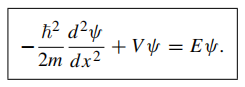
The time-independent Schrodinger equation
Reason for considering separable wave functions:
They are stationary states, i.e., the probability density \(|\Psi|^2=|\psi(x)|^2\) is time-independent. The same thing holds for the expectation of any dynamic variable.
They are states of definite total energy. The Hamiltonian (kinetic plus potential): \[ H(x,p)=\frac{p^2}{2m}+V(x), \] has a corresponding Hamiltonian operator by substituting \(p\) with \(-i\hbar\frac \partial{\partial t}\).
Thus the time-independent Schrodinger equation can be written \(\hat H\psi=E\psi\).
- Expectation is \(\langle H\rangle=E\), with \(\langle H^2\rangle=E^2\).
- Variance of \(H\) is \(\sigma_H^2=0\).
The general solution is a linear combination of separable solutions.
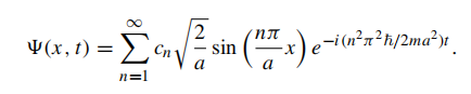
Different energies (allowed energy) \(\{E_n\}\) correspond to different wave functions. \[ \Psi(x,t)=\sum_{n=1}^\infty c_n\psi_n(x)e^{-iE_nt/\hbar} \] is also a solution to Schrodinger equation.
The physical meaning of \(\{c_n\}\).
\(|c_n|^2\) is the probability that a measurement of the energy would return the value \(E_n\).
- \[ \sum_{n=1}^\infty|c_n|^2=1,\langle H\rangle=\sum_{n=1}^\infty|c_n|^2E_n. \]
The infinite square well
Suppose \[ V(x)=\left\{\begin{array}{cc} 0, & 0\le x\le a,\\ \infty, & \text{otherwise} \end{array}\right. \]
By \(\psi(0)=\psi(a)=0\), and normalization requirement, we have \[ \psi_n(x)=\sqrt{\frac 2a}\sin(\frac{n\pi}ax),\text{ and }E_n=\frac{n^2\pi^2\hbar^2}{2ma^2}. \]
\(\psi_1\) with the lowest energy is called the ground state, while the others are called excited states.
Properties of \(\psi_n\)
They are alternately even and odd w.r.t. the center of the well.
\(\int\psi_m^*\psi_ndx=\delta_{mn}\).
They're complete. \(\forall f(x)\), it can be expressed as \[ f(x)=\sum_{n=1}^\infty c_n\psi_n(x),\text{ where }c_n=\int\psi_n(x)^*f(x)dx. \]
The general solution to Schrodinger equation:
The harmonic oscillator
Chapter 3 | Formalism
Hilbert space
The set of all square-integrable functions, on a specified interval constitutes a vector space \(L^2(a,b)\), or Hilbert space. \[ f(x)\text{ s.t. }\int_a^b|f(x)|^2dx<\infty. \]
Inner product of two functions \(f,g\) is \(\langle f|g\rangle=\int_a^bf^*g\ dx\).
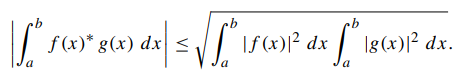
Schwarz inequality:
Observables
Observables are represented by hermitian operators.
Hermitian conjugate (or adjoint) of an operator \(\hat Q\) is \(\hat Q^\dagger\) s.t. \[ \langle f|\hat Qg\rangle=\langle \hat Q^\dagger f|g\rangle,\forall f,g. \]
Hermitian operator satisfies \(\hat Q=\hat Q^\dagger\).
Determinate states: every measurement of \(Q\) is certain to return the same value, say, \(q\).
- Determinate states of \(Q\) are eigenfunctions of \(\hat Q\).
- All eigenvalues of \(Q\) is called its spectrum.
If two or more eigenfunctions share the same eigenvalue, the spectrum is said to be degenerate.
Eigenfunctions of a hermitian operator
- Eigenvalues of a Hermitian are real.
- Eigenfunctions of a Hermitian belonging to distinct eigenvalues are orthogonal.
- Axiom: the eigenfunctions of an observable operator are complete: any function (in Hilbert space) can be expressed as a linear combination of them.
- If a spectrum of a hermitian operator is continuous, the eigenfunctions are not normalizable, they're not in Hilbert space and don't represent possible physical states.
Generalized statistical interpretation
If we measure an observable \(Q(x,p)\), on a particle in the state \(\Psi(x,t)\), we are certain to get one of the eigenvalues of the hermitian operator \(\hat Q(x,-i\hbar d/dx)\).
Note that classical variables \(x,p\) commute while \(\hat x,\hat p\) don't commute. Luckily, observables containing the multiplication of \(x,p\) are rare, but when they do occur some other consideration must be invoked to resolve the ambiguity.
If the spectrum of \(\hat Q\) is discrete, the probability of getting eigenvalue \(q_n\) associated with the orthonormal eigenfunction \(f_n(x)\) is \(|\langle f_n|\Psi\rangle|^2\). If the spectrum is continuous, with real eigenvalues \(q(z)\) and Dirac-orthonormal eigenfunction \(f_z(x)\), the probability of getting a result in the range \(dz\) is \(|\langle f_z|\Psi\rangle|^2dz\).
The momentum space wave function \(\Phi\) is \[ \Phi(p,t)=c(p)=\langle f_p|\Psi\rangle=\frac 1{\sqrt{2\pi\hbar}}\int_{-\infty}^\infty e^{-ipx/\hbar}\Psi(x,t)dx,\\ \text{and the inverse Fourier transform is }\Psi(x,t)=\frac 1{\sqrt{2\pi\hbar}}\int_{-\infty}^\infty e^{ipx/\hbar}\Phi(p,t)dp. \] The eigenfunctions of momentum operator is \(f_p=\frac{1}{\sqrt{2\pi\hbar}}e^{ipx/\hbar}\).
The uncertainty principle
- Proof of the generalized uncertainty principle
For any observable \(A\), we have \[ \sigma_A^2=\langle (\hat A-\langle A\rangle)|(\hat A-\langle A\rangle)\Psi\rangle\triangleq \langle f|f\rangle. \] Similarly \(\sigma_B^2=\langle g|g\rangle\). Therefore by Schwarz inequality \[ \sigma_A^2\sigma_B^2=\langle f|f\rangle\langle g|g\rangle\ge |\langle f|g\rangle|^2. \] For any \(z\in \mathbb C\), \[ |z|^2\ge \text{Im}^2(z)=[\frac 1{2i}(z-z^*)]^2. \] Let \(z=\langle f|g\rangle\), we have \[ \sigma_A^2\sigma_B^2\ge \left(\frac 1{2i}\left[\langle f|g\rangle-\langle g|f\rangle\right]\right)^2. \] Using the hermicity of \((\hat A-\langle A\rangle)\), we have \[ \langle f|g\rangle=\langle \hat A\hat B\rangle-\langle A\rangle\langle B\rangle. \] So \[ \langle f|g\rangle-\langle g|f\rangle=\langle \hat A\hat B\rangle-\langle \hat B\hat A\rangle=\langle [\hat A,\hat B]\rangle. \] Combining the above results, we have \[ \bf \sigma_A^2\sigma_B^2\ge \left(\frac 1{2i}\left\langle \left[\hat A,\hat B\right]\right\rangle\right)^2. \]
The minimum-uncertainty wave packet
The sufficient and necessary condition for reaching the minimum of uncertainty inequality is \[ g(x)=iaf(x),a\in \mathbb R. \]
Common uncertainty principle
Position-momentum \[ \Delta x\Delta p\ge \frac \hbar 2. \]
Energy-time \[ \Delta t\Delta E\ge \frac \hbar 2. \]
- Note that for an observable \(Q\), we have
 The Schrodinger equation says \[
i\hbar \frac{\partial \Psi}{\partial t}=\hat H\Psi,
\] so
The Schrodinger equation says \[
i\hbar \frac{\partial \Psi}{\partial t}=\hat H\Psi,
\] so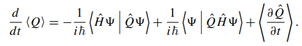 But \(\hat H\) is hermitian, so
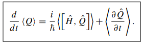 Now pick \(A=H,B=Q\), and suppose the observable doesn't depend explicitly on time, \[
\sigma_H\sigma_Q\ge \frac \hbar 2\left|\frac{d\langle Q\rangle}{dt}\right|.
\] Define \(\Delta E=\sigma_H,\Delta t=\frac{\sigma_Q}{|d\langle Q\rangle / dt}|\), we can get the energy-time uncertainty principle.
Now pick \(A=H,B=Q\), and suppose the observable doesn't depend explicitly on time, \[
\sigma_H\sigma_Q\ge \frac \hbar 2\left|\frac{d\langle Q\rangle}{dt}\right|.
\] Define \(\Delta E=\sigma_H,\Delta t=\frac{\sigma_Q}{|d\langle Q\rangle / dt}|\), we can get the energy-time uncertainty principle.- Here \(\Delta t\) represents the amount of time it takes the expectation value of \(Q\) to change by one standard deviation, not an average of measurement on time!
Vectors and operators
Chapter 4 | Quantum Mechanics in 3D
Chapter 5 | Identical Particles
Two-particle systems
The state of a 2-particle system is \[ \Psi(\vec r_1,\vec r_2,t). \] The Hamiltonian for the whole system is \[ \hat H=-\frac{\hbar^2}{2m_1}\nabla_1^2-\frac{\hbar^2}{2m_2}\nabla_2^2+V(\vec r_1,\vec r_2,t). \]
- There're 2 special cases we can reduce the time-independent Schrodinger equation to one-particle problem:
- Noninteracting particles, \(V(\vec r_1,\vec r_2)= V_1(\vec r_1)+V_2(\vec r_2)\).
- Central potentials, \(V(\vec r_1,\vec r_2)=V(|\vec r_1-\vec r_2|)\).
All electrons are utterly identical. One can't tell an electron from another.
In quantum mechanics, we can construct a wave function that is noncommittal as to which particle is in which state, i.e., \[ \psi_\pm(\vec r_1,\vec r_2)=A[\psi_a(\vec r_1)\psi_b(\vec r_2)\pm \psi_b(\vec r_1)\psi_a(\vec r_2)]; \] the theory admits 2 kinds of identical particles: bosons(with plus sign) and fermions(with minus sign).
- All particles with integer spin are bosons, and all particles with half integer spin are fermions.
Pauli exclusion principle: It follows that two identical fermions cannot occupy the same state, otherwise \(\psi_-(\vec r_1,\vec r_2)\) will be zero.
Exchange force
If two particles are distinguishable, and number 1 is in state \(\psi_a\), then the combined wave function is \[ \psi(x_1,x_2)=\psi_a(x_1)\psi_b(x_2); \] if they are identical particles, the composition wave function is \[ \psi_\pm(x_1,x_2)=\frac 1{\sqrt 2}[\psi_a(x_1)\psi_b(x_2)\pm \psi_b(x_1)\psi_a(x_2)]. \] Consider the value $(x_1-x_2)^2$,
For distinguishable particles, \[ \langle (\Delta x)^2\rangle _d=\langle x^2\rangle_a+\langle x^2\rangle_b -2\langle x\rangle_a\langle x\rangle_b. \]
For identical particles, \[ \langle (\Delta x)^2\rangle_\pm=\langle x^2\rangle_a+\langle x^2\rangle_b -2\langle x\rangle_a\langle x\rangle_b\mp 2|\langle x\rangle_{ab}|^2. \]
Note that identical bosons tend to be somewhat closer, and identical fermions somewhat farther apart, than distinguishable particles in the same two states. It's like some "force" makes such effects, which is called exchange force.
Spin
- Actually we need to consider the spin of two particles, and get state \(\psi(\vec r_1,\vec r_2)\chi(1,2)\).
Pauli principle actually allows two electrons in a given position state, as long as their spins are in the singlet configuration.